The Kimi team recently dropped the Attention Residuals paper. The core idea extends residual connections with an attention mechanism that attends across layers rather than tokens. This gives the model learned control over how it composes information across depth.
I wanted to play around with this on a budget, so I forked nanoGPT and added AttnRes. There's already been a lot of activity reproducing the results, so feel free to skip to the results I found compelling beyond the base repro:
- Per-token routing patterns
- Designing annealing schedules (+ adaptive block boundaries)
- Interactions with value residuals
Building up to AttnRes
Residual connections have evolved since their original introduction in the transformer paper:
- The original transformer used PostNorm, which normalizes after the residual addition: . This keeps hidden state magnitudes bounded, but placing normalization directly on the residual path leads gradients to vanish at high depth (multiplying a non-identity Jacobian per layer). This is why the original transformer required LR warmup, allowing gradients to settle before taking larger steps.
- PreNorm was an improvement over PostNorm, normalizing the input to each layer instead: . PreNorm made deep transformers dramatically easier to train and became the universal default. But with nothing constraining the residual stream magnitude (nothing constraints the layer output term!), hidden state magnitudes grow with depth + later layers learn to produce larger outputs so they can affect the residual stream. This progressively dilutes each early layer's relative contribution (denoted PreNorm dilution).
- There have been attempts to learn a scalar per layer to address PreNorm dilution. Variations of from papers like LayerScale, DeepNorm, and FixUp. These efforts haven't demonstrated compelling gains at modern LLM scales, so vanilla PreNorm remains the default.
Kimi's approach replaces the fixed residual accumulation with learned depth attention. Each layer gets a query vector (low param cost; only parameters each) that computes softmax attention over all previous layer outputs:
I extracted the vector out to make the types / dims of each term clearer. The softmax is applied to the vector of values, so the weights sum to 1. Each layer constructs its input as a weighted average over all previous layer outputs.
The model can now learn which historical layers matter for each subsequent computation (as a result of being learned). Standard attention attends across tokens at a single layer. AttnRes attends across layers for a single token.
This is also interesting from a mech interp perspective. The residual stream is a useful proxy for studying transformer internals, and AttnRes gives us more explicit weights showing us how each layer composes information from previous layers.
Implementation
The full AttnRes module is ~70 lines of PyTorch.
RMSNorm: Before computing depth attention, we normalize each layer's output by its root-mean-square. Without this, layers that naturally produce larger outputs would dominate the softmax regardless of whether their content is actually relevant. This is the same reason attention over tokens uses scaling, but applied to the depth dimension instead.
Zero-initialized queries: Each layer's query vector starts at zero. Since , the model begins by uniformly averaging all previous layer outputs. Over training, the queries specialize and the model learns to route.
Two variants: Full AttnRes applies depth attention at every layer, allowing the model to learn which layers are most relevant for each subsequent computation. Block AttnRes groups layers into blocks (we used 4 blocks of 3 layers on nanoGPT), applies normal PreNorm residuals within each block, and only does depth attention at block boundaries.
Training setup
Three runs on Modal A100-40GBs, all identical except for the residual mode (baseline vs block AttnRes vs full AttnRes):
- GPT-2 124M (12 layers, 768 dim, 12 heads)
- OpenWebText dataset
- 10K training steps, batch size 12, 5 gradient accumulation steps
- AdamW, cosine LR schedule, 6e-4 peak LR
Cost ~$15 across all three runs. Training took about 3 hours per run. Tracked results with W&B.
Results
I'll walk through some of the noisy results first, then get into the interesting stuff.
The loss improvement is marginal. At step 10K, baseline lands at 3.478, full AttnRes lands at 3.456, and Block AttnRes sits at 3.474. Full AttnRes has the lowest loss, but small diffs across the board.
Makes sense at 12 layers. The paper's gains (7.5 points on GPQA-Diamond) came from a 48B parameter MoE model with far more layers. With our GPT-2 124M depth, the PreNorm dilution problem isn't severe enough for AttnRes to make a big difference in loss.
Training dynamics
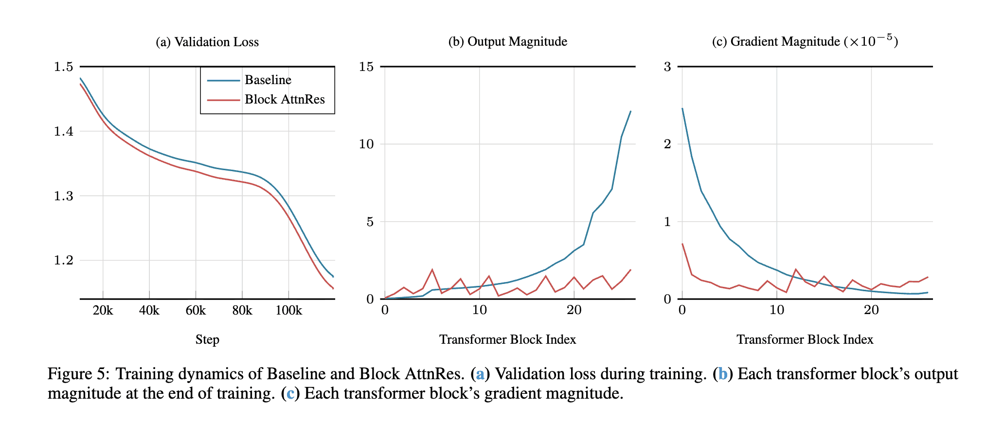
The paper's Figure 5 shows AttnRes bounding representation magnitudes at scale (copied here for convenience). Output magnitudes increase with depth and gradient magnitudes start high and drop off with depth in the baseline. Block AttnRes bounds the output magnitudes and gradients.
In our reproduction with 12 layers, the picture is messier. Full AttnRes (orange) flattens the middle layers (2–10), but spikes at layer 12 (70, higher than baseline's 49). Block AttnRes (green) spikes at layer 1 (100) then drops. Gradient magnitudes (right) are noisy across all variants.
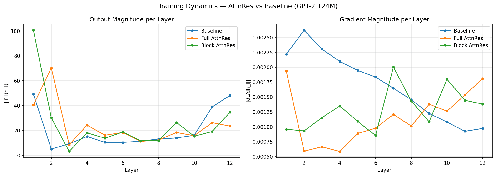
At this depth, AttnRes just changes where magnitude concentrates rather than uniformly bounding it. The paper's cleaner results come from 100+ layer models where the dilution problem is actually severe. Noisy results at this scale, expected.
Depth attention heatmaps
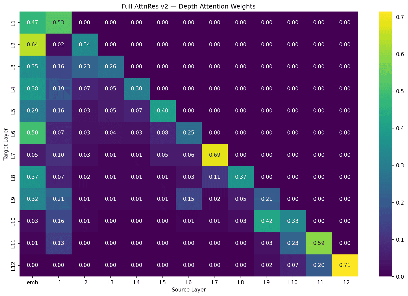
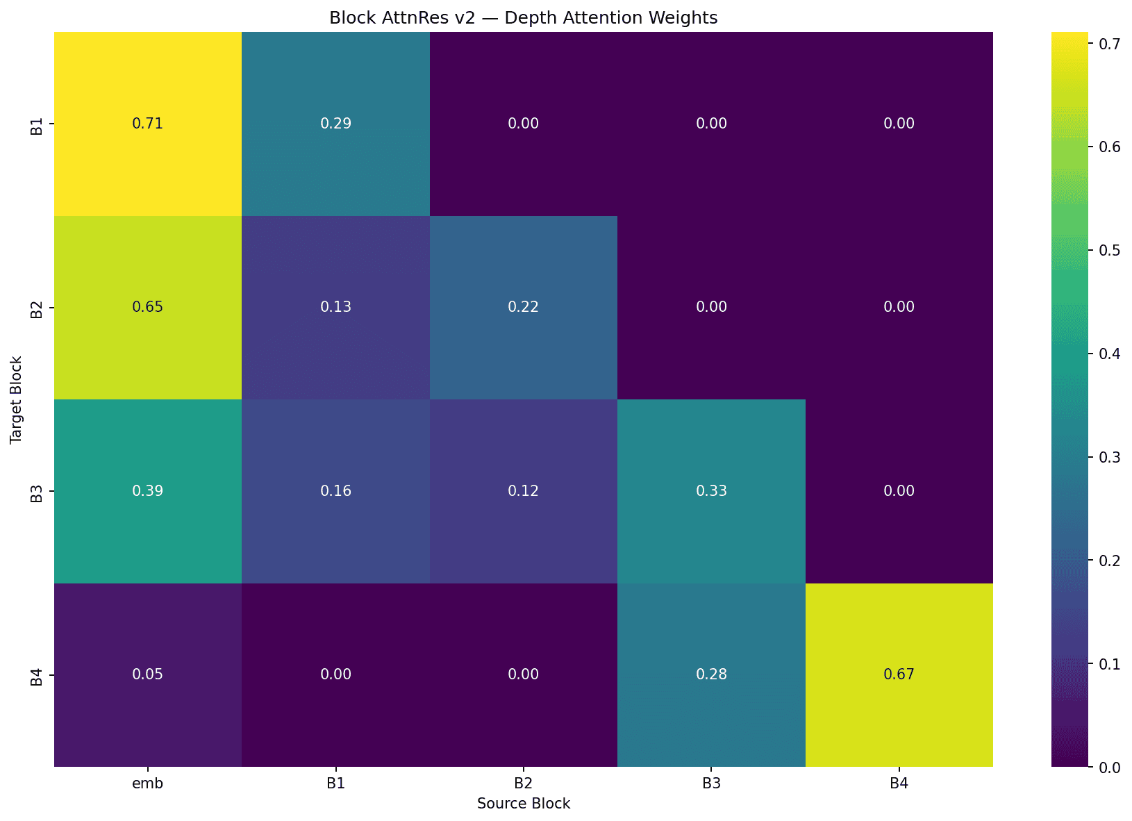
Each cell shows how much layer/block (row) attends to the output of each other layer/block (column). Here's full AttnRes (per-layer) and block AttnRes (4 blocks of 3 layers):
The same patterns appear in both, just at different granularity:
Self-attention bias: Most layers attend heavily to their own output or the most recent output. In full AttnRes, L7 → L7 at 0.69 and L12 → L12 at 0.71. In block AttnRes, B1 → emb at 0.71 and B4 → B4 at 0.67.
Embedding persistence: Early layers/blocks attend strongly to the raw embedding. Full AttnRes L1–L6 put 29–64% on the embedding, dropping at L7 and L10 onwards. Block AttnRes shows the same: B1-B3 at 0.71, 0.65, and 0.39, then fading to 0.05 by B4.
Learned skip connections: Not every layer attends to its immediate predecessor. In full AttnRes, L9 reaches back to the embedding (0.32) and L6 (0.15), skipping intermediate layers. L1 is useful for most later layers. In block AttnRes, B3 spreads attention across emb (0.39), B1 (0.16), B2 (0.12), and B3 (0.33) which is a broad mix rather than just the previous block.
Query vector similarity
Each layer's is a learned pseudo-query that determines how that layer weighs its sources via dot product with the keys. Cosine similarity between pairs of vectors tells us which layers learned similar routing strategies. Negative cosine similarity means two layers are looking for opposite things.
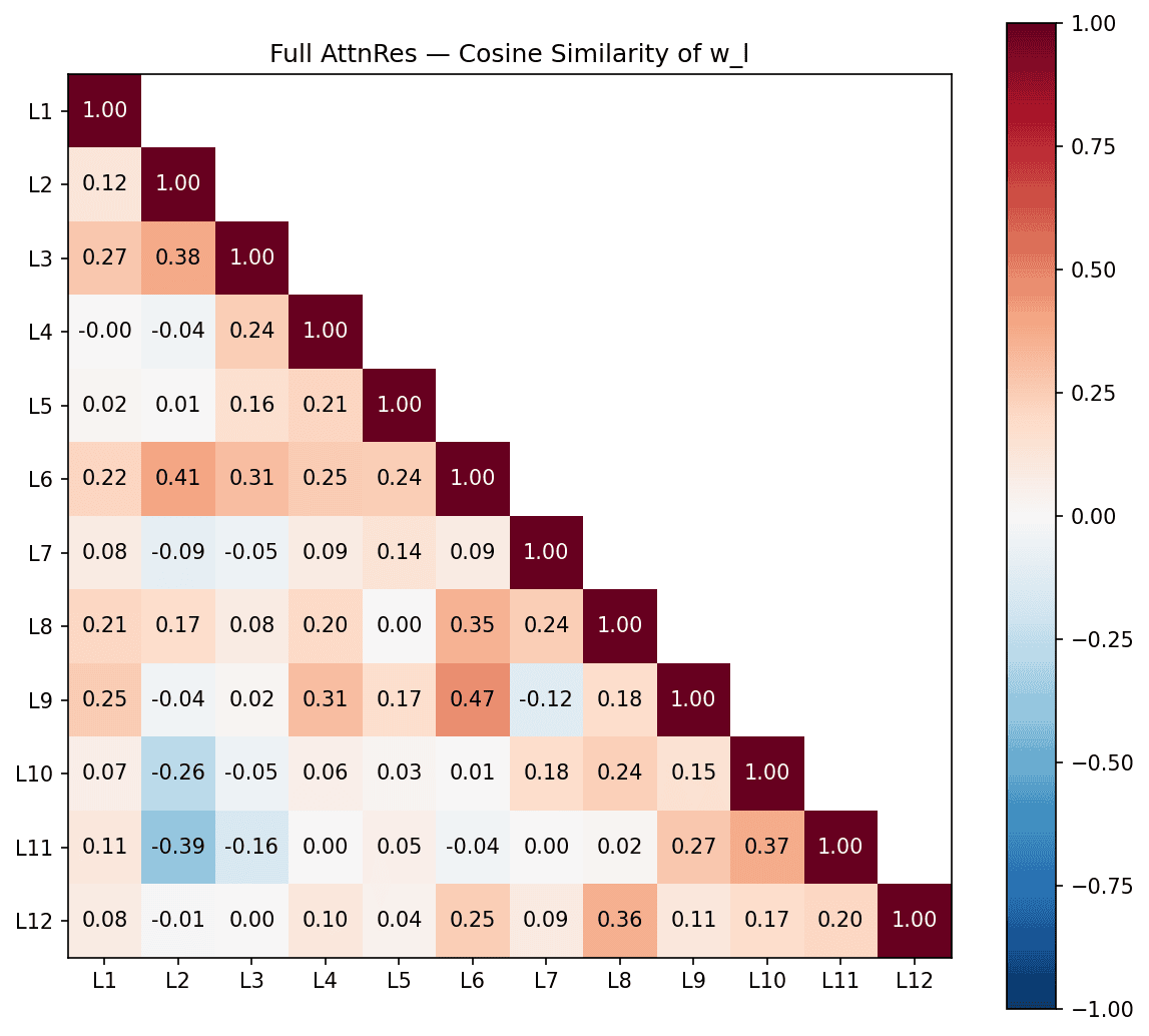
In full AttnRes, a few pairs stand out. The most similar are L6–L9 (0.47), suggesting these two layers use very similar routing strategies despite being 3 layers apart. L2–L6 (0.41) is strong pair.
L2–L11 (-0.39) is the strongest negative pair: an early layer and a late layer actively looking for opposite things. L2–L10 (-0.26) shows the same pattern.
L2 is a polarizing query vector. It's similar to its neighbors (L3, L6) but becomes increasingly anti-correlated with the last few layers (L10, L11). The model learns an early-vs-late split in what information it routes.
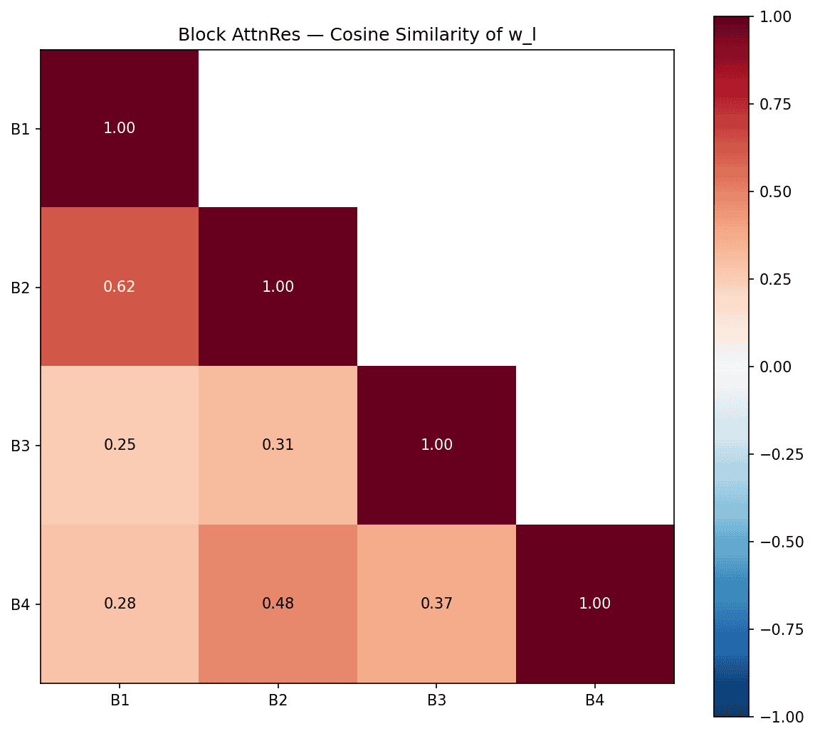
There's a simpler story with Block AttnRes. With only 4 blocks, all pairwise similarities are positive (0.25–0.62), with B1–B2 at 0.62 being the most similar. There's less room for specialization and opposition as you see in the 12-layer version.
Token routing patterns
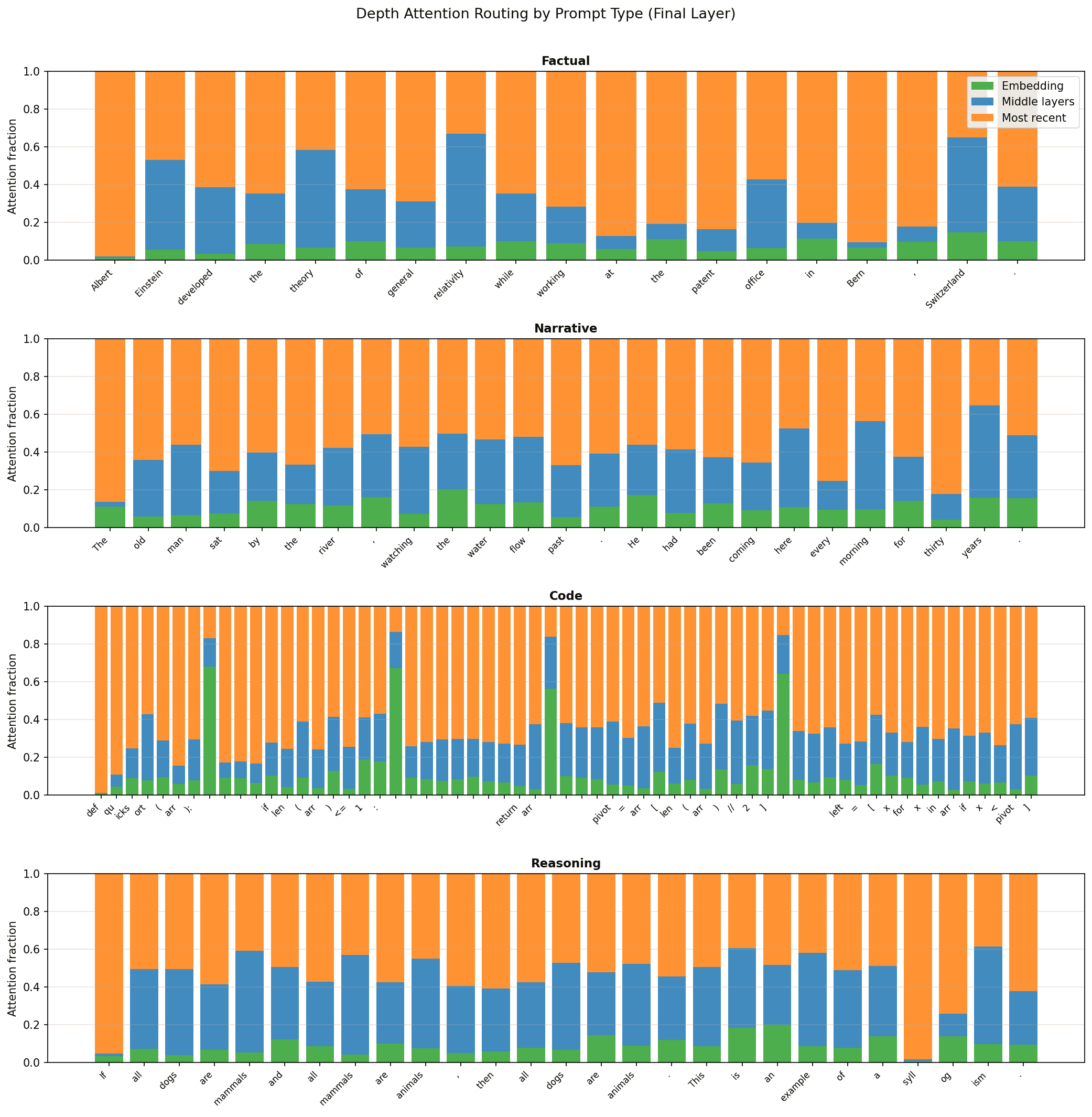
The learned query vector gives us a window into how the model routes information across depth for each token. I wanted to explore this across different types of content. I split prompts into four categories (factual, narrative, coding, and reasoning) and visualized the depth attention weights at the final block boundary.
The routing didn't look that visually interesting at first. It was uniform across prompt categories (full figure in appendix). The only interesting pattern visually was with the code regime.
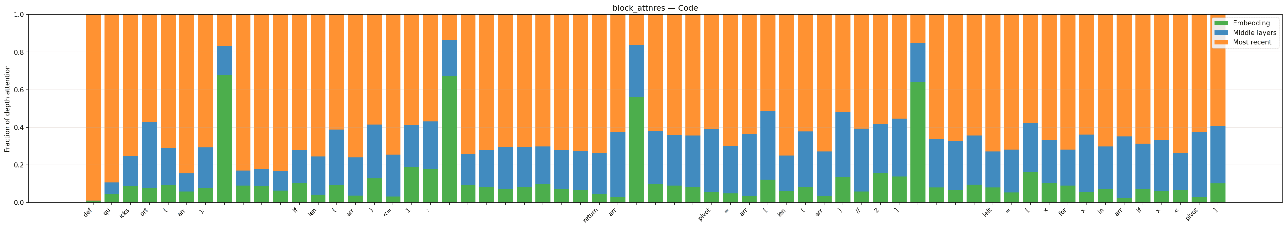
Embedding attention spikes at structural boundary tokens: newlines, syntax delimiters like :, [, ], (, ), and keywords like if. These are the points where the model is about to transition between syntactic units.
Interior tokens, like the ones inside arr[len(arr)//2], lean harder on middle layers. This makes intuitive sense. At a boundary token, the model faces a "what kind of token comes next?" question. The embedding layer provides the strongest signal. Mid-expression, the question shifts to asking about surrounding tokens for syntax.
A quick follow up to this. We were only looking at the final block boundary. What about the intermediate blocks? We visualized the depth attention weights at each intermediate block given the quicksort prompt.
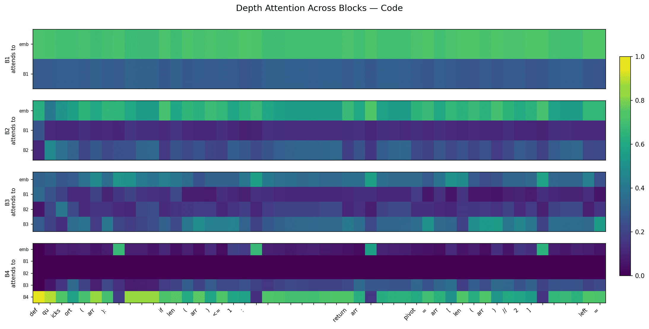
This figure shows depth attention weights at each of the 4 block boundaries, for every token in the quicksort prompt. B1 attends almost entirely to the embedding. B2 and B3 progressively mix in earlier block outputs. The "reset to embedding" pattern from the stacked bar chart shows up specifically at B4. The model develops the syntax routing only at the last block boundary, where it most directly affects the output.
Full AttnRes shows a similar pattern at middle layers (particularly L7) rather than the final layer. By L12, embedding attention is near zero for all tokens. The signal is noisier with 12 layers of routing, but the same structure in middle layers suggests this may be a property of depth attention.
This is only reproduced on a small 124M model, so it would be interesting to see if this sharpens with scale and code specific training.
Branching off AttnRes
Experimenting is cheap and fast these days. I brainstormed with Claude to figure out good extension directions (autoresearch FTW).
Same setup throughout: GPT-2 124M on OpenWebText, 10K steps.
Experiment 1: Adaptive Block Boundaries
Idea: Block AttnRes uses fixed, uniform block boundaries: 4 blocks of 3 layers each in our case. But every block is the same size. Maybe the model wants more frequent depth attention in the early layers where embedding information is flowing, and less in the late layers where representations are more settled.
Instead of hardcoding block positions, we add a learnable "boundary logit" between every pair of adjacent layers. A sigmoid gate determines whether that position is a block boundary. Temperature annealing lets the model explore softly early in training (), then snap to hard 0/1 decisions late in training (). A regularization term gently encourages ~4 boundaries. Code snippet here.
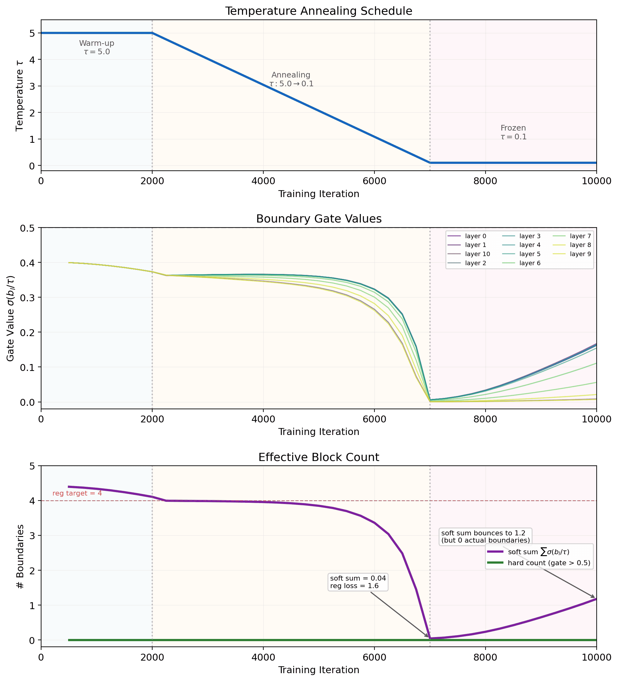
The model eliminates all boundaries. Every gate collapses toward 0 as temperature anneals, and the effective block count drops from ~4 to near zero. The brief bounce-back after iter 7000 is due to the regularization term pushing gates back up when is far from its target of 4. The model clearly prefers no boundaries.
This confirms what the original paper already showed: full AttnRes > block AttnRes. The result should have been obvious from the start given the paper's claims (a bit of oversight on my part), but still cool to see the claim confirmed empirically via a learned parameter.
There's a couple further experiments I'd like to run here. Discussed in the summary.
Experiment 2: Value Residual Learning
Value Residual Learning (Zhou et al., 2025) addresses a related problem to AttnRes. In standard transformers, each layer computes fresh Q, K, V projections from the current hidden state. The values determine what information gets mixed after attention. By deep layers, the values have been recomputed from scratch so many times that the original token-level information is gone from the value stream. Value residual learning mixes each layer's computed values with (the first layer's value projection), giving deep layers persistent access to raw token information.
In each attention layer, they replace the computed values with a weighted mix:
They use a per-layer learnable lambda, initialized at 0.5. We implemented with nanoGPT here.
At GPT-2 scale, value residuals alone slightly hurt performance (3.483 vs baseline's 3.478). Twelve layers isn't deep enough for value stream dilution to be a real problem, and the forced mixing with seems to add noise. Adding value residuals to Block AttnRes produced no improvement whatsoever (3.475 vs 3.474). Value residuals are a hardcoded solution to a problem AttnRes learns to handle on its own.
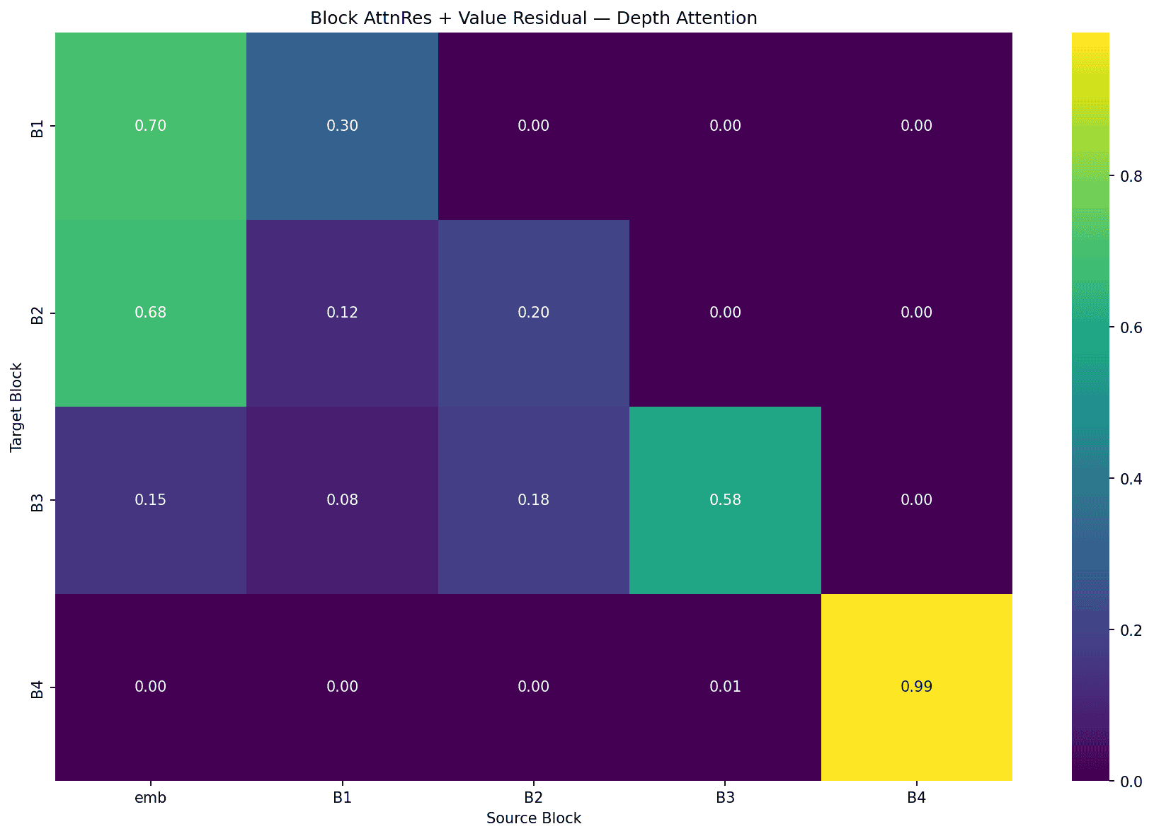
When value residuals are present, depth attention becomes dramatically more biased towards recency. B4 goes from 0.67 (with just Block AttnRes) to 0.99 (with value residuals) self-attention, nearly ignoring all earlier layers.
This connects to the embedding persistence we observed in the AttnRes depth heatmaps. The model discovers, through learned attention over depth, the same insight that the value residual paper engineered more directly. Deep layers prefer access to raw token information.
Summary + future experiments
At GPT-2 124M scale, the AttnRes loss improvements are marginal, but the mechanism reveals interesting structure: embedding persistence in early layers, learned skip connections, and token-type specific routing patterns in code. Value residuals address a related problem but become redundant when AttnRes is present. Adaptive block boundaries confirmed the paper's finding that full AttnRes dominates block AttnRes.
A couple future directions to explore (most are towards scaling):
- More mech interp experiments on the code token routing stuff. Different languages and at larger scale.
- Increase layer depth to see if we can determine where PreNorm dilution hurts. Maybe deeper models with a smaller hidden dim could isolate the depth effect from scale?
- Test different temperature annealing schedules to see if we can get better adaptive boundary behavior. Maybe forcing some minimum number of boundaries to see if boundaries end up evenly distributed? Or having the initialization biased more towards boundaries, rather than starting at ~0.4?
And some random thoughts throughout the process:
- Claude messed up on the scaling in the PyTorch implementation. Cost $15, bad Claude.
- Understanding the lineage of ideas (the evolution from PostNorm → PreNorm → scalar stuff → AttnRes) has always helped my learning. LLMs make this much easier.
- Things are easier to implement than ever. Papers are best interacted with by reproducing them.
If you made it this far, thanks for reading! I wrote this to help my understanding and I hope it's useful for others too.
Appendix
Token routing patterns by prompt type
We split prompts into four categories (factual, narrative, coding, and reasoning) and visualized the depth attention weights at the final block boundary. Across all categories (except code), the routing looks uniform.
Expanding the residual formula
Just for fun. The AttnRes notation seemed simple enough. And I added KaTeX to this site recently, let's expand:
Expanding gives us a cleaner view of what's happening, but the core intuition already exists in the original formula: the dot product is a similarity measure between the per-layer query and each previous layer output . This expansion also shows us that RMSNorm strips the magnitude from the attention weights entirely, so only direction determines how much to attend. This is also pretty intuitive because of RMSNorm's definition, but it's nice to see it explicitly. The sharpness of this selection is controlled by , which acts as an inverse temperature on the softmax.
Shoutout Claude, Modal, W&B. I wrote most of the words here. Code / visuals generated with Claude.